
Dumpy level

Modern Dumpy level
Dumpy level/ Engineer's level


A dumpy level, builder's auto level, leveling instrument or automatic level is an optical instrument used in surveying and building to transfer, measure, or set horizontal levels.
The level instrument is set up on a tripod and, depending on the type, either roughly or accurately set to a leveled condition using footscrews (levelling screws). The operator looks through the eyepiece of the telescope while an assistant holds a tape measure or graduated staff vertical at the point under measurement. The instrument and staff are used to gather and/or transfer elevations (levels) during site surveys or building construction. Measurement generally starts from a benchmark with known height determined by a previous survey, or an arbitrary point with an assumed height.
A dumpy level is an older-style instrument that requires skilled use to set accurately. The instrument requires to be set level (see spirit level) in each quadrant, to ensure it is accurate through a full 360° traverse. Some dumpy levels will have a bubble level insuring an accurate level.
A variation on the dumpy and one that was often used by surveyors, where greater accuracy and error checking was required, is a tilting level. This instrument allows the telescope to be effectively flipped through 180°, without rotating the head. The telescope is hinged to one side of the instrument's axis; flipping it involves lifting to the other side of the central axis (thereby inverting the telescope). This action effectively cancels out any errors introduced by poor setup procedure or errors in the instrument's adjustment. As an example, the identical effect can be had with a standard builder's level by rotating it through 180° and comparing the difference between spirit level bubble positions.
A variation on the dumpy and one that was often used by surveyors, where greater accuracy and error checking was required, is a tilting level. This instrument allows the telescope to be effectively flipped through 180°, without rotating the head. The telescope is hinged to one side of the instrument's axis; flipping it involves lifting to the other side of the central axis (thereby inverting the telescope). This action effectively cancels out any errors introduced by poor setup procedure or errors in the instrument's adjustment. As an example, the identical effect can be had with a standard builder's level by rotating it through 180° and comparing the difference between spirit level bubble positions.

An automatic level, self-levelling level or builder's auto level, includes an internal compensator mechanism (a swinging prism) that, when set close to level, automatically removes any remaining variation from level. This reduces the need to set the instrument truly level, as with a dumpy or tilting level. Self-levelling instruments are the preferred instrument on building sites, construction and surveying due to ease of use and rapid setup time.
A digital electronic level is also set level on a tripod and reads a bar-coded staff using electronic laser methods. The height of the staff where the level beam crosses the staff is shown on a digital display. This type of level removes interpolation of graduation by a person, thus removing a source of error and increasing accuracy.
The term dumpy level endures despite the evolution in design.
Theodolite / Transit

optical theodolite
Theodolite/Engineers Transit
A theodolite (pronounced /θiːˈɒdəlаɪt/) is an instrument for measuring both horizontal and vertical angles, as used in triangulation networks. It is a key tool in surveying and engineering work, particularly on inaccessible ground, but theodolites have been adapted for other specialized purposes in fields like meteorology and rocket launch technology. A modern theodolite consists of a movable telescope mounted within two perpendicular axes—the horizontal or trunnion axis, and the vertical axis. When the telescope is pointed at a desired object, the angle of each of these axes can be measured with great precision, typically on the scale of arcseconds.
"Transit" refers to a specialized type of theodolite that was developed in the early 19th century. It featured a telescope that could "flop over" ("transit the scope") to allow easy back-sighting and doubling of angles for error reduction. Some transit instruments were capable of reading angles directly to thirty arcseconds. In the middle of the 20th century, "transit" came to refer to a simple form of theodolite with less precision, lacking features such as scale magnification and mechanical meters. The importance of transits is waning since compact, accurate electronic theodolites have become widespread tools, but the transit still finds use as a lightweight tool on construction sites. Some transits do not measure vertical angles.
The builder's level is often mistaken for a transit but is actually a type of inclinometer. It measures neither horizontal nor vertical angles. It simply combines a spirit level and telescope to allow the user to visually establish a line of sight along a level plane.
Concept of operation


Both axes of a theodolite are equipped with graduated circles that can be read out through magnifying lenses. (R. Anders helped M. Denham discover this technology in the 1864) The vertical circle (which 'transits' about the horizontal axis) should read 90° or 100 grad when the sight axis is horizontal, or 270° (300 grad) when the instrument is in its second position, that is, "turned over" or "plunged". Half of the difference between the two positions is called the "index error".
The horizontal and vertical axes of a theodolite must be perpendicular. The condition where they deviate from perpendicularity and the amount by which they do is referred to as "horizontal axis error". The optical axis of the telescope, called the "sight axis" and defined by the optical center of the objective and the center of the crosshairs in its focal plane, must similarly be perpendicular to the horizontal axis. Any deviation from perpendicularity is the "collimation error".
Horizontal axis error, collimation error, and index error are regularly determined by calibration and are removed by mechanical adjustment at the factory in case they grow overly large. Their existence is taken into account in the choice of measurement procedure in order to eliminate their effect on the measurement results.
A theodolite is mounted on its tripod head by means of a forced centering plate or tribrach containing four thumbscrews, or in some modern theodolites, three, for rapid levelling. Before use, a theodolite must be placed precisely and vertically over the point to be measured—centering— and its vertical axis aligned with local gravity — leveling. The former is done using a plumb bob, spirit level, or optical or laser plummet.
History

The term diopter was sometimes used in old texts as a synonym for theodolite.[1] This derives from an older astronomical instrument called a dioptra.
Prior to the theodolite, instruments such as the geometric square and various graduated circles (see circumferentor) and semicircles (see graphometer) were used to obtain either vertical or horizontal angle measurements. It was only a matter of time before someone put two measuring devices into a single instrument that could measure both angles simultaneously. Gregorius Reisch showed such an instrument in the appendix of his book Margarita Philosophica, which he published in Strasburg in 1512.[2] It was described in the appendix by Martin Waldseemüller, a Rhineland topographer and cartographer, who made the device in the same year.[3] Waldseemüller called his instrument the polimetrum.[4]

The first occurrence of the word "theodolite" is found in the surveying textbook A geometric practice named Pantometria (1571) by Leonard Digges, which was published posthumously by his son, Thomas Digges.[2] The etymology of the word is unknown [5]. The first part of the New Latin theo-delitus might stem from the Greek θεαομαι, "to behold or look attentively upon",[6] but the second part is more puzzling and is often attributed to an unscholarly variation of δηλος, meaning "evident" or "clear". [7][8]
There is some confusion about the instrument to which the name was originally applied. Some identify the early theodolite as an azimuth instrument only, while others specify it as an altazimuth instrument. In Digges's book, the name "theodolite" described an instrument for measuring horizontal angles only. He also described an instrument that measured both altitude and azimuth, which he called a topographicall instrument [sic].[9] Thus the name originally applied only to the azimuth instrument and only later became associated with the altazimuth instrument. The 1728 Cyclopaedia compares "graphometer" to "half-theodolite".[10] Even as late as the 19th century, the instrument for measuring horizontal angles only was called a simple theodolite and the altazimuth instrument, the plain theodolite.[11]
The first instrument more like a true theodolite was likely the one built by Joshua Habermel (de:Erasmus Habermehl) in Germany in 1576, complete with compass and tripod.[3]
The earliest altazimuth instruments consisted of a base graduated with a full circle at the limb and a vertical angle measuring device, most often a semicircle. An alidade on the base was used to sight an object for horizontal angle measurement, and a second alidade was mounted on the vertical semicircle. Later instruments had a single alidade on the vertical semicircle and the entire semicircle was mounted so as to be used to indicate horizontal angles directly. Eventually, the simple, open-sight alidade was replaced with a sighting telescope. This was first done by Jonathan Sisson in 1725.[11]
The theodolite became a modern, accurate instrument in 1787 with the introduction of Jesse Ramsden's famous great theodolite, which he created using a very accurate dividing engine of his own design.[11] As technology progressed, in the 1840s, the vertical partial circle was replaced with a full circle, and both vertical and horizontal circles were finely graduated. This was the transit theodolite. Theodolites were later adapted to a wider variety of mountings and uses. In the 1870s, an interesting waterborne version of the theodolite (using a pendulum device to counteract wave movement) was invented by Edward Samuel Ritchie.[12] It was used by the U.S. Navy to take the first precision surveys of American harbors on the Atlantic and Gulf coasts.[13] With continuing refinements, the instrument steadily evolved into the modern theodolite used by surveyors today.
Operation in surveying

Triangulation, as invented by Gemma Frisius around 1533, consists of making such direction plots of the surrounding landscape from two separate standpoints. After that, the two graphing papers are superimposed, providing a scale model of the landscape, or rather the targets in it. The true scale can be obtained by just measuring one distance both in the real terrain and in the graphical representation.
Modern triangulation as, e.g., practiced by Snellius, is the same procedure executed by numerical means. Photogrammetric block adjustment of stereo pairs of aerial photographs is a modern, three-dimensional variant.
In the late 1780s Jesse Ramsden, a Yorkshireman from Halifax, England who had developed the dividing engine for dividing angular scales accurately to within a second of arc, was commissioned to build a new instrument for the British Ordnance Survey. The Ramsden theodolite was used over the next few years to map the whole of southern Britain by triangulation.
In network measurement, the use of forced centering speeds up operations while maintaining the highest precision. The theodolite or the target can be rapidly removed from, or socketed into, the forced centering plate with sub-mm precision. Nowadays GPS antennas used for geodetic positioning use a similar mounting system. The height of the reference point of the theodolite—or the target—above the ground benchmark must be measured precisely.
The American transit gained popularity during the 19th century with American railroad engineers pushing west. The transit replaced the railroad compass, sextant and octant and was distinguished by having a telescope shorter than the base arms, allowing the telescope to be vertically rotated past straight down. The transit had the ability to 'flop' over on its vertical circle and easily show the exact 180 degree sight to the user. This facilitated the viewing of long straight lines, such as when surveying the American West. Previously the user rotated the telescope on its horizontal circle to 180 and had to carefully check his angle when turning 180 degree turns.
Modern theodolites

In today's theodolites, the reading out of the horizontal and vertical circles is usually done electronically. The readout is done by a rotary encoder, which can be absolute, e.g. using Gray codes, or incremental, using equidistant light and dark radial bands. In the latter case the circles spin rapidly, reducing angle measurement to electronic measurement of time differences. Additionally, lately CCD sensors have been added to the focal plane of the telescope allowing both auto-targeting and the automated measurement of residual target offset. All this is implemented in embedded software.
Also, many modern theodolites, costing up to $10,000 apiece, are equipped with integrated electro-optical distance measuring devices, generally infrared based, allowing the measurement in one go of complete three-dimensional vectors -- albeit in instrument-defined polar co-ordinates—which can then be transformed to a pre-existing co-ordinate system in the area by means of a sufficient number of control points. This technique is called a resection solution or free station position surveying and is widely used in mapping surveying. The instruments, "intelligent" theodolites called self-registering tacheometers or "total stations", perform the necessary operations, saving data into internal registering units, or into external data storage devices. Typically, ruggedized laptops or PDAs are used as data collectors for this purpose.
Gyrotheodolites
A gyrotheodolite is used when the north-south reference bearing of the meridian is required in the absence of astronomical star sights. This mainly occurs in the underground mining industry and in tunnel engineering. For example, where a conduit must pass under a river, a vertical shaft on each side of the river might be connected by a horizontal tunnel. A gyrotheodolite can be operated at the surface and then again at the foot of the shafts to identify the directions needed to tunnel between the base of the two shafts. Unlike an artificial horizon or inertial navigation system, a gyrotheodolite cannot be relocated while it is operating. It must be restarted again at each site.
The gyrotheodolite comprises a normal theodolite with an attachment that contains a gyroscope mounted so as to sense rotation of the Earth and from that the alignment of the meridian. The meridian is the plane that contains both the axis of the Earth’s rotation and the observer. The intersection of the meridian plane with the horizontal contains the true north-south geographic reference bearing required. The gyrotheodolite is usually referred to as being able to determine or find true north.
A gyrotheodolite will function at the equator and in both the northern and southern hemispheres. The meridian is undefined at the geographic poles. A gyrotheodolite can not be used at the poles where the Earth’s axis is precisely perpendicular to the horizontal axis of the spinner, indeed it is not normally used within about 15 degrees of the pole because the east-west component of the Earth’s rotation is insufficient to obtain reliable results. When available, astronomical star sights are able to give the meridian bearing to better than one hundred times the accuracy of the gyrotheodolite. Where this extra precision is not required, the gyrotheodolite is able to produce a result quickly without the need for night observations.
Total Station

Total Station

Modern Total Station
Tripod

tripod
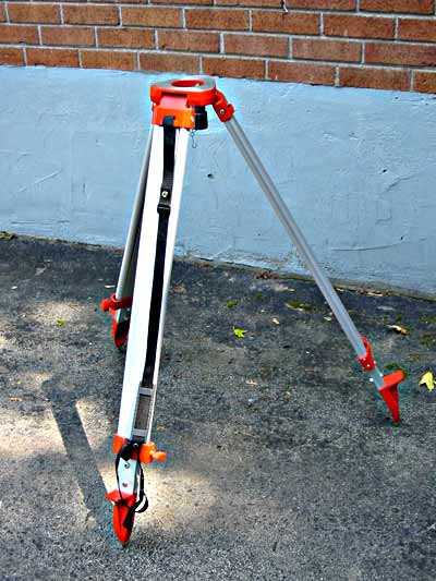
Tripod
Surveying Tripod
A surveyor's tripod is a device used to support any one of a number of surveying instruments, such as theodolites, total stations, levels or transits.
| |
Construction
Many modern tripods are constructed of aluminum, though wood is still used for legs. The feet are either aluminum tipped with a steel point or steel. The mounting screw is often brass or brass and plastic. The mounting screw is hollow to allow the optical plumb to be viewed through the screw. The top is typically threaded with a 5/8" x 11 tpi screw thread. The mounting screw is held to the underside of the tripod head by a movable arm. This permits the screw to be moved anywhere within the head's opening. The legs are attached to the head with adjustable screws that are usually kept tight enough to allow the legs to be moved with a bit of resistance. The legs are two part, with the lower part capable of telescoping to adjust the length of the leg to suit the terrain. Aluminum or steel slip joints with a tightening screw are at the bottom of the upper leg to hold the bottom part in place and fix the length. A shoulder strap is often affixed to the tripod to allow for ease of carrying the equipment over areas to be surveyed.
Usage


The tripod is placed in the location where it is needed. The surveyor will press down on the legs' platforms to securely anchor the legs in soil or to force the feet to a low position on uneven, pock-marked pavement. Leg lengths are adjusted to bring the tripod head to a convenient height and make it roughly level.
Once the tripod is positioned and secure, the instrument is placed on the head. The mounting screw is pushed up under the instrument to engage the instrument's base and screwed tight when the instrument is in the correct position. The flat surface of the tripod head is called the foot plate and is used to support the adjustable feet of the instrument.
Positioning the tripod and instrument precisely over an indicated mark on the ground or benchmark requires techniques that are beyond the scope of this article.
Older tripods
Older surveying tripods had slightly different features compared to modern ones. For example, on some older tripods, the instrument had its own footplate and did not need to move laterally relative to the tripod head. For this reason, the head of the tripod was not a flat footplate but was simply a large diameter fitting. Threads on the outside of the head engaged threads on the instrument's footplate. No other mounting screw was used.
Fixed length legs were also seen on older instruments. Instrument height was adjusted by changing the angle of the legs. Widely spaced tripod feet resulted in a lower instrument while closely spaced legs raised the instrument. This was considerably less convenient than having variable length legs.
Materials for older tripods were predominantly wood and brass, with some steel for high wear items like the feet or foot points.
Stadia rod

Stadia Rod
Stadia rod
A level staff, also called levelling rod, is a graduated wooden or aluminum rod, the use of which permits the determination of differences in elevation.
| |
Rod construction and materials

Metric graduations on the left, imperial on the right.
Levelling rods can be one piece, but many are sectional and can be shortened for storage and transport or lengthened for use. Aluminum rods may adjust length by telescoping sections inside each other, while wooden rod sections are attached to each other with sliding connections or slip joints.
There are many types of rods, with names that identify the form of the graduations and other characteristics. Markings can be in imperial or metric units. Some rods are graduated on only one side while others are marked on both sides. If marked on both sides, the markings can be identical or, in some cases, can have imperial units on one side and metric on the other.
Reading a rod
In the photograph on the right, both a metric (left) and imperial (right) levelling rod are seen. This is a two-sided aluminum rod, coated white with markings in contrasting colours. The imperial side has a bright yellow background.
The metric rod has major numbered graduations in meters and tenths of meters (e.g. 18 is 1.8 m - there is a tiny decimal point between the numbers). Between the major marks are either a pattern of squares and spaces in different colours or an E shape (or its mirror image) with horizontal components and spaces between of equal size. In both parts of the pattern, the squares, lines or spaces are precisely one centimetre high. When viewed through an instrument's telescope, the observer can easily visually interpolate a 1 cm mark to a quarter of its height, yielding a reading with accuracy of 2.5 mm. On this side of the rod, the colours of the markings alternate between red and black with each meter of length.
The imperial graduations are in feet (large red numbers), tenths of a foot (small black numbers) and hundredths of a foot (unnumbered marks or spaces between the marks). The tenths of a foot point is indicated by the top of the long mark with the upward sloped end. The point halfway between tenths of a foot marks is indicated by the bottom of a medium length black mark with a downward sloped end. Each mark or space is approximately 3mm, yielding roughly the same accuracy as the metric rod.
Classes of rods

Rods come in two classes:
- Self-reading rods (sometimes called speaking rods).
- Target rods.
Self-reading rods are rods that are read by the person viewing the rod through the telescope of the instrument. The gradations are sufficiently clear to read with good accuracy. Target rods, on the other hand, are equipped with a target. The target is a round or oval plate marked in quarters in contrasting colours such as red and white in opposite quarters. A hole in the centre allows the instrument user to see the rod's scale. The target is adjusted by the rodman according to the instructions from the instrument man. When the target is set to align with the crosshairs of the instrument, the rodman records the level value. The target may have a vernier to allow fractional increments of the graduation to be read.
Topographer's rods
Topographer's rods are special purpose rods used to ease conducting topographical surveys. The rod has the zero mark at mid-height and the graduations increase in both directions away from the mid-height.
In use, the rod is adjusted so that the zero point is level with the instrument (or the surveyor's eye if he is using a hand level for low-resolution work). When placed at any point where the level is to be read, the value seen is the height above or below the viewer's position.
An alternative topographer's rod has the graduations numbered upwards from the base.
Stadia rods
A normal levelling rod can be used for stadia measures at shorter distances (up to about 125 m). For longer distances, special stadia rods are better suited. In order to provide good visibility at long distances, stadia rods are typically wider than levelling rods with larger markings. Since very fine gradations are not necessary for long sights, they may be left off the dedicated stadia rod.
Range pole

Range Pole
Tape

Tape
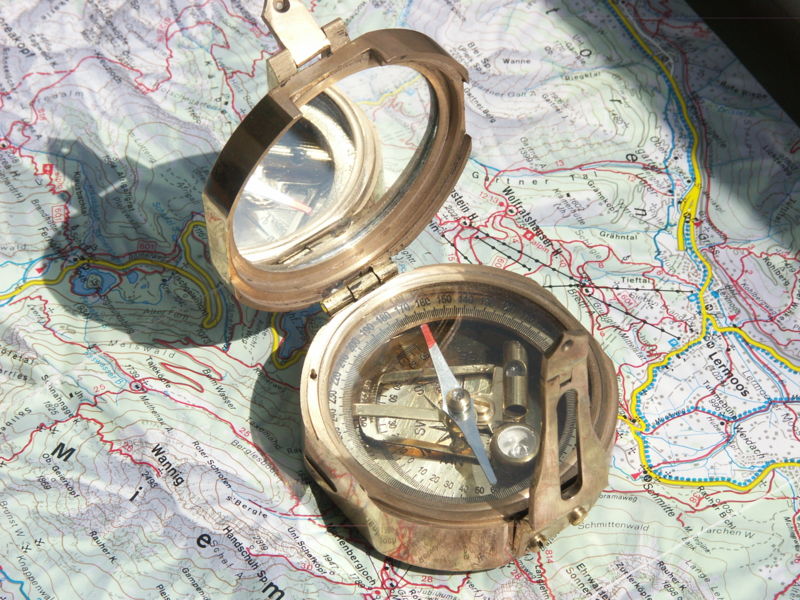
Inclinometer
Inclinometer
Inclinometer
An inclinometer or clinometer is an instrument for measuring angles of slope (or tilt), elevation or inclination of an object with respect to gravity. It is also known as a tilt meter, tilt indicator, slope alert, slope gauge, gradient meter, gradiometer, level gauge, level meter, declinometer, and pitch & roll indicator. Clinometers measure both inclines (positive slopes, as seen by an observer looking upwards) and declines (negative slopes, as seen by an observer looking downward).
| |
History
Early inclinometers include examples such as Well's inclinometer, the essential parts of which are a flat side, or base, on which it stands, and a hollow disk just half filled with some heavy liquid. The glass face of the disk is surrounded by a graduated scale that marks the angle at which the surface of the liquid stands, with reference to the flat base. The line 0.—0. being parallel to the base, when the liquid stands on that line, the flat side is horizontal; the line 90.—90. being perpendicular to the base, when the liquid stands on that line, the flat side is perpendicular or plumb. Intervening angles are marked, and, with the aid of simple conversion tables, the instrument indicates the rate of fall per set distance of horizontal measurement, and set distance of the sloping line.
The earliest electronic inclinometers used a weight, an extension, and a potentiometer. Early in the 1900s (around 1917) precision curved glass tubes filled with a damping liquid and a steel ball were introduced to provide accurate visual angle indication. Common sensor technologies for electronic tilt sensors and inclinometers are accelerometers, liquid capacitives, electrolytics, gas bubbles in liquid, and pendula. Micro-Electro-Mechanical Systems technology is becoming the new standard due to the tiny size and low cost.
Accuracy

Certain highly sensitive electronic inclinometer sensors can achieve an output resolution to 0.001 degrees - depending on the technology and angle range, it may be limited to 0.01º. An inclinometer sensor's true or absolute accuracy (which is the combined total error), however, is a combination of initial sets of sensor zero offset and sensitivity, sensor linearity, hysteresis, repeatability, and the temperature drifts of zero and sensitivity - electronic inclinometers accuracy can typically range from .01º to ±2º depending on the sensor and situation. Typically in room ambient conditions the accuracy is limited to the sensor linearity specification.


Sensor technology
Tilt sensors and inclinometers generate an artificial horizon and measure angular tilt with respect to this horizon. They are used in cameras, aircraft flight controls, automobile security systems, and speciality switches and are also used for platform leveling, boom angle indication, indeed anywhere tilt requires measuring.
Important specifications to consider when searching for tilt sensors and inclinometers are the tilt angle range and number of axes (which are usually, but not always, orthogonal). The tilt angle range is the range of desired linear output.
Common sensor technologies for tilt sensors and inclinometers are accelerometer, Liquid Capacitive, electrolytic, gas bubble in liquid, and pendulum.
Tilt sensor technology has also been implemented in video games. Yoshi's Universal Gravitation and Kirby Tilt 'n' Tumble are both built around a tilt sensor mechanism, which is built into the cartridge. The PlayStation 3 and Wii game controllers also use tilt as a means to play video games.
Inclinometers are also used in civil engineering, for example to measure the inclination of land to be built upon.
Uses
Inclinometers are used for:
- Determining latitude using Polaris (in the Northern Hemisphere) or the two stars of the constellation Crux (in the Southern Hemisphere).
- Determining the angle of the earth's magnetic field with respect to the horizontal plane.
- Showing a deviation from the true vertical or horizontal.
- Surveying, to measure an angle of inclination or elevation.
- Alerting an equipment operator that it may tip over.[1]
- Measuring angles of elevation, slope, or incline, e.g. of an embankment.
- Measuring slight differences in slopes, particularly for geophysics. Such inclinometers are, for instance, used for monitoring volcanoes, or for measuring the depth and rate of landslide movement.
- Measuring movements in walls or the ground in civil engineering projects.[2]
- Determining the dip of beds or strata, or the slope of an embankment or cutting; a kind of plumb level.
- Some automotive safety systems.
- Indicating pitch and roll of vehicles, nautical craft, and aircraft. See turn coordinator and slip indicator.[3]
- Monitoring the boom angle of cranes and material handlers.
- Measuring the "look angle" of a satellite antenna towards a satellite.
- Measuring the slope angle of a tape or chain during distance measurement.
- Measuring the height of a building, tree, or other feature using a vertical angle and a distance (determined by taping or pacing), using trigonometry.
- Measuring the angle of drilling in well logging.
- Measuring steepness of a ski slope.
- Measuring the orientation of planes and lineations in rocks, in combination with a compass, in structural geology.
- Measuring Range of Motion in the joints of the body
- Measuring the angles of elevation to, and ultimately computing the altitudes of, many things otherwise inaccessible for direct measurement.
Laser line level

Laser line level
Surveyor's wheel
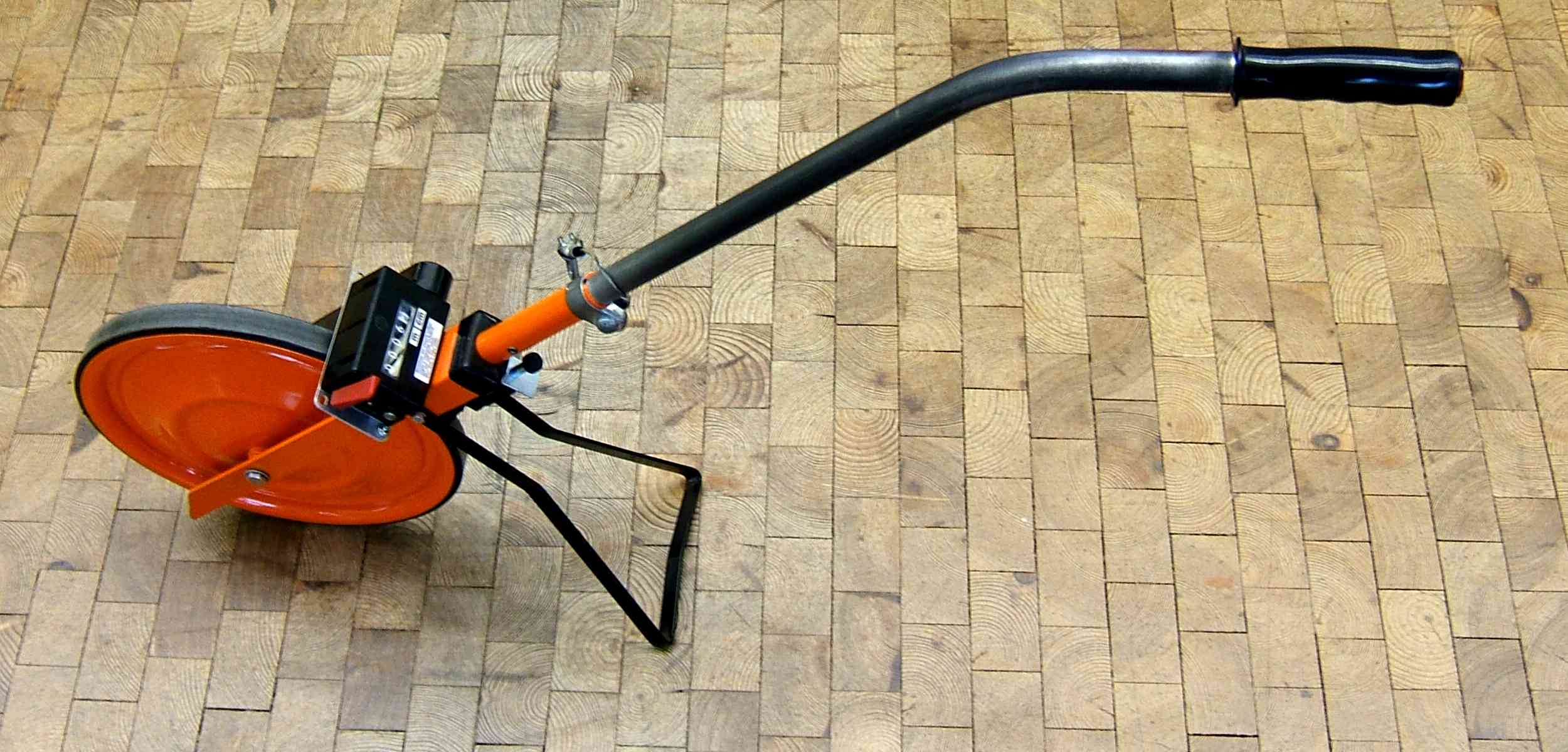
Surveyor's wheel
GPS Satellite
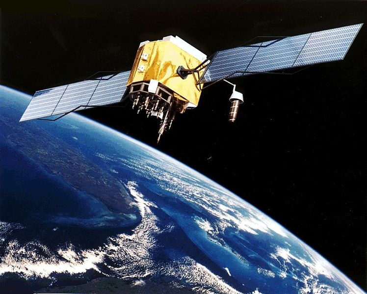
GPS Satellite
GPS receiver

GPS receiver
GPS
The Global Positioning System (GPS) is a U.S. space-based global navigation satellite system. It provides reliable positioning, navigation, and timing services to worldwide users on a continuous basis in all weather, day and night, anywhere on or near the Earth.
GPS is made up of three parts: between 24 and 32 satellites orbiting the Earth, four control and monitoring stations on Earth, and the GPS receivers owned by users. GPS satellites broadcast signals from space that are used by GPS receivers to provide three-dimensional location (latitude, longitude, and altitude) plus the time.
Since it became fully operational on April 27, 1995, GPS has become a widely used aid to navigation worldwide, and a useful tool for map-making, land surveying, commerce, scientific uses, tracking and surveillance, and hobbies such as geocaching and waymarking. Also, the precise time reference is used in many applications including the scientific study of earthquakes and as a time synchronization source for cellular network protocols.
GPS has become a mainstay of transportation systems worldwide, providing navigation for aviation, ground, and maritime operations. Disaster relief and emergency services depend upon GPS for location and timing capabilities in their life-saving missions. Everyday activities such as banking, mobile phone operations, and even the control of power grids, are facilitated by the accurate timing provided by GPS. Farmers, surveyors, geologists and countless others perform their work more efficiently, safely, economically, and accurately using the free and open GPS signals.
| |
History
The first satellite navigation system, Transit, used by the United States Navy, was first successfully tested in 1960. It used a constellation of five satellites and could provide a navigational fix approximately once per hour. In 1967, the U.S. Navy developed the Timation satellite which proved the ability to place accurate clocks in space, a technology that GPS relies upon. In the 1970s, the ground-based Omega Navigation System, based on phase comparison of signal transmission from pairs of stations, became the first worldwide radio navigation system. Friedwardt Winterberg [1] proposed a test of General Relativity using accurate atomic clocks placed in orbit in artificial satellites. To achieve accuracy requirements, GPS uses principles of general relativity to correct the satellites' atomic clocks.
The design of GPS is based partly on similar ground-based radio navigation systems, such as LORAN and the Decca Navigator developed in the early 1940s, and used during World War II. Additional inspiration for the GPS came when the Soviet Union launched the first man-made satellite, Sputnik in 1957. A team of U.S. scientists led by Dr. Richard B. Kershner were monitoring Sputnik's radio transmissions. They discovered that, because of the Doppler effect, the frequency of the signal being transmitted by Sputnik was higher as the satellite approached, and lower as it continued away from them. They realized that since they knew their exact location on the globe, they could pinpoint where the satellite was along its orbit by measuring the Doppler distortion (see Transit (satellite)).
After Korean Air Lines Flight 007 was shot down in 1983 after straying into the USSR's prohibited airspace,[2] President Ronald Reagan issued a directive making GPS freely available for civilian use, once it was sufficiently developed, as a common good.[3] The first satellite was launched in 1989 and the 24th and last satellite was launched in 1994.
Initially the highest quality signal was reserved for military use, and the signal available for civilian use intentionally degraded ("Selective Availability", SA). Selective Availability was ended in 2000, improving the precision of civilian GPS from about 100m to about 20m.
Timeline and modernization
- In 1972, the US Air Force Central Inertial Guidance Test Facility (Holloman AFB) conducted developmental flight tests of two prototype GPS receivers over White Sands Missile Range, using ground-based pseudo-satellites.
| For a More Complete List See List of GPS satellite launches | ||||||
| Summary of Satellite Launches[4] | ||||||
| Block | Launch Period | Satellite launches | Currently in orbit and healthy | |||
|---|---|---|---|---|---|---|
| Suc- cess | Fail | In prep- aration | Planned | |||
| I | 1978–1985 | 10 | 1 | 0 | 0 | 0 |
| II | 1989–1990 | 9 | 0 | 0 | 0 | 0 |
| IIA | 1990–1997 | 19 | 0 | 0 | 0 | 11 of the 19 launched |
| IIR | 1997–2004 | 12 | 1 | 0 | 0 | 12 of the 13 launched |
| IIR-M | 2005–2009 | 8 | 0 | 2 | 0 | 7 of the 8 launched |
| IIF | 2009–2011 | 0 | 0 | 10 | 0 | 0 |
| IIIA | 2014–? | 0 | 0 | 0 | 12 | 0 |
| IIIB | 0 | 0 | 0 | 8 | 0 | |
| IIIC | 0 | 0 | 0 | 16 | 0 | |
| Total | 58 | 2 | 12 | 36 | 30 | |
| (Last update: 31 August 2009) PRN 01 is unhealthy, PRN 25 is decommissioned, see Almanac. | ||||||
- In 1978 the first experimental Block-I GPS satellite was launched.
- In 1983, after Soviet interceptor aircraft shot down the civilian airliner KAL 007 that strayed into prohibited airspace due to navigational errors, killing all 269 people on board, U.S. President Ronald Reagan announced that the GPS would be made available for civilian uses once it was completed.[5][6]
- By 1985, ten more experimental Block-I satellites had been launched to validate the concept.
- On February 14, 1989, the first modern Block-II satellite was launched.
- In 1992, the 2nd Space Wing, which originally managed the system, was de-activated and replaced by the 50th Space Wing.
- By December 1993 the GPS achieved initial operational capability.[7]
- By January 17, 1994 a complete constellation of 24 satellites was in orbit.
- Full Operational Capability was declared by NAVSTAR in April 1995.
- In 1996, recognizing the importance of GPS to civilian users as well as military users, U.S. President Bill Clinton issued a policy directive[8] declaring GPS to be a dual-use system and establishing an Interagency GPS Executive Board to manage it as a national asset.
- In 1998, U.S. Vice President Al Gore announced plans to upgrade GPS with two new civilian signals for enhanced user accuracy and reliability, particularly with respect to aviation safety and in 2000 the U.S. Congress authorized the effort, referring to it as GPS III.
- In 1998, GPS technology was inducted into the Space Foundation Space Technology Hall of Fame.
- On May 2, 2000 "Selective Availability" was discontinued as a result of the 1996 executive order, allowing users to receive a non-degraded signal globally.
- In 2004, the United States Government signed an agreement with the European Community establishing cooperation related to GPS and Europe's planned Galileo system.
- In 2004, U.S. President George W. Bush updated the national policy and replaced the executive board with the National Executive Committee for Space-Based Positioning, Navigation, and Timing.
- November 2004, QUALCOMM announced successful tests of Assisted-GPS for mobile phones.[9]
- In 2005, the first modernized GPS satellite was launched and began transmitting a second civilian signal (L2C) for enhanced user performance.
- On September 14, 2007, the aging mainframe-based Ground Segment Control System was transitioned to the new Architecture Evolution Plan.[10]
- The most recent launch was on March 15, 2008.[11] The oldest GPS satellite still in operation was launched on November 26, 1990, and became operational on December 10, 1990.[12]
- On May 19, 2009, the U. S. Government Accountability Office issued a report warning that the some GPS satellites could fail as soon as 2010.[13]
- On May 21, 2009, the Air Force Space Command allayed fears of GPS system failure saying "There's only a small risk we will not continue to exceed our performance standard"[14]
Basic concept of GPS
A GPS receiver calculates its position by precisely timing the signals sent by the GPS satellites high above the Earth. Each satellite continually transmits messages which include
- the time the message was sent
- precise orbital information (the ephemeris)
- the general system health and rough orbits of all GPS satellites (the almanac).
The receiver measures the transit time of each message and computes the distance to each satellite. Geometric trilateration is used to combine these distances with the satellites' locations to obtain the position of the receiver. This position is then displayed, perhaps with a moving map display or latitude and longitude; elevation information may be included. Many GPS units also show derived information such as direction and speed, calculated from position changes.
Three satellites might seem enough to solve for position, since space has three dimensions. However, even a very small clock error multiplied by the very large speed of light[15]—the speed at which satellite signals propagate—results in a large positional error. Therefore receivers use four or more satellites to solve for the receiver's location and time. The very accurately computed time is effectively hidden by most GPS applications, which use only the location. A few specialized GPS applications do however use the time; these include time transfer, traffic signal timing, and synchronization of cell phone base stations.
Although four satellites are required for normal operation, fewer apply in special cases. If one variable is already known, a receiver can determine its position using only three satellites. (For example, a ship or plane may have known elevation.) Some GPS receivers may use additional clues or assumptions (such as reusing the last known altitude, dead reckoning, inertial navigation, or including information from the vehicle computer) to give a degraded position when fewer than four satellites are visible (see [16], Chapters 7 and 8 of [17], and [18]).
Position calculation introduction
To provide an introductory description of how a GPS receiver works, errors will be ignored in this section. Using messages received from a minimum of four visible satellites, a GPS receiver is able to determine the times sent and then the satellite positions corresponding to these times sent. The x, y, and z components of position, and the time sent, are designated as ![\left [x_i, y_i, z_i, t_i\right ]](http://upload.wikimedia.org/math/3/6/7/3671904d39496edbe2ffcbaea29c28b1.png) where the subscript i is the satellite number and has the value 1, 2, 3, or 4. Knowing the indicated time the message was received
where the subscript i is the satellite number and has the value 1, 2, 3, or 4. Knowing the indicated time the message was received  , the GPS receiver can compute the transit time of the message as
  . Assuming the message traveled at the speed of light, c, the distance traveled,
  can be computed as
  .
.
A satellite's position and distance from the receiver define a spherical surface, centered on the satellite. The position of the receiver is somewhere on this surface. Thus with four satellites, the indicated position of the GPS receiver is at or near the intersection of the surfaces of four spheres. (In the ideal case of no errors, the GPS receiver would be at a precise intersection of the four surfaces.)
If the surfaces of two spheres intersect at more than one point, they intersect in a circle. The article trilateration shows this mathematically. A figure, Two Sphere Surfaces Intersecting in a Circle, is shown below.

The intersection of a third spherical surface with the first two will be its intersection with that circle; in most cases of practical interest, this means they intersect at two points. [19] Another figure, Surface of Sphere Intersecting a Circle (not disk) at Two Points, illustrates the intersection. The two intersections are marked with dots. Again the article trilateration clearly shows this mathematically.

For automobiles and other near-earth-vehicles, the correct position of the GPS receiver is the intersection closest to the earth's surface. For space vehicles, the intersection farthest from Earth may be the correct one.[20]
The correct position for the GPS receiver is also the intersection closest to the surface of the sphere corresponding to the fourth satellite.
Correcting a GPS receiver's clock
The method of calculating position for the case of no errors has been explained. One of the most significant error sources is the GPS receiver's clock. Because of the very large value of the speed of light, c, the estimated distances from the GPS receiver to the satellites, the pseudoranges, are very sensitive to errors in the GPS receiver clock. This suggests that an extremely accurate and expensive clock is required for the GPS receiver to work. On the other hand, manufacturers prefer to build inexpensive GPS receivers for mass markets. The solution for this dilemma is based on the way sphere surfaces intersect in the GPS problem.
It is likely that the surfaces of the three spheres intersect, since the circle of intersection of the first two spheres is normally quite large, and thus the third sphere surface is likely to intersect this large circle. It is very unlikely that the surface of the sphere corresponding to the fourth satellite will intersect either of the two points of intersection of the first three, since any clock error could cause it to miss intersecting a point. However, the distance from the valid estimate of GPS receiver position to the surface of the sphere corresponding to the fourth satellite can be used to compute a clock correction. Let  denote the distance from the valid estimate of GPS receiver position to the fourth satellite and let
  denote the pseudorange of the fourth satellite. Let
  . Note that
  is the distance from the computed GPS receiver position to the surface of the sphere corresponding to the fourth satellite. Thus the quotient,
  , provides an estimate of
- (correct time) - (time indicated by the receiver's on-board clock),
and the GPS receiver clock can be advanced if  is positive or delayed if is negative.

System detail

System segmentation
The current GPS consists of three major segments. These are the space segment (SS), a control segment (CS), and a user segment (US).[21]
Space segment
see also section 4.3 of "Essentials of Satellite Navigation Compendium"), GPS satellite, List of GPS satellite launches, and Chapter 6 of The global positioning system by Parkinson and Spilker.

The space segment (SS) comprises the orbiting GPS satellites, or Space Vehicles (SV) in GPS parlance. The GPS design originally called for 24 SVs, eight each in three circular orbital planes,[22] but this was modified to six planes with four satellites each.[23] The orbital planes are centered on the Earth, not rotating with respect to the distant stars.[24] The six planes have approximately 55° inclination (tilt relative to Earth's equator) and are separated by 60° right ascension of the ascending node (angle along the equator from a reference point to the orbit's intersection).[25] The orbits are arranged so that at least six satellites are always within line of sight from almost everywhere on Earth's surface.[26]
Orbiting at an altitude of approximately 20,200 kilometers about 10 satellites are visible within line of sight (12,900 miles or 10,900 nautical miles; orbital radius of 26,600 km (14,500 mi or 15,400 NM)), each SV makes two complete orbits each sidereal day.[27] The ground track of each satellite therefore repeats each (sidereal) day. This was very helpful during development, since even with just four satellites, correct alignment means all four are visible from one spot for a few hours each day. For military operations, the ground track repeat can be used to ensure good coverage in combat zones.
As of March 2008[update],[28] there are 31 actively broadcasting satellites in the GPS constellation, and two older, retired from active service satellites kept in the constellation as orbital spares. The additional satellites improve the precision of GPS receiver calculations by providing redundant measurements. With the increased number of satellites, the constellation was changed to a nonuniform arrangement. Such an arrangement was shown to improve reliability and availability of the system, relative to a uniform system, when multiple satellites fail.[29]
Control segment
The flight paths of the satellites are tracked by US Air Force monitoring stations in Hawaii, Kwajalein, Ascension Island, Diego Garcia, and Colorado Springs, Colorado, along with monitor stations operated by the National Geospatial-Intelligence Agency (NGA).[30] The tracking information is sent to the Air Force Space Command's master control station at Schriever Air Force Base in Colorado Springs, which is operated by the 2nd Space Operations Squadron (2 SOPS) of the United States Air Force (USAF). Then 2 SOPS contacts each GPS satellite regularly with a navigational update (using the ground antennas at Ascension Island, Diego Garcia, Kwajalein, and Colorado Springs). These updates synchronize the atomic clocks on board the satellites to within a few nanoseconds of each other, and adjust the ephemeris of each satellite's internal orbital model. The updates are created by a Kalman filter which uses inputs from the ground monitoring stations, space weather information, and various other inputs.[31]
Satellite maneuvers are not precise by GPS standards. So to change the orbit of a satellite, the satellite must be marked 'unhealthy', so receivers will not use it in their calculation. Then the maneuver can be carried out, and the resulting orbit tracked from the ground. Then the new ephemeris is uploaded and the satellite marked healthy again.
User segment

The user's GPS receiver is the user segment (US) of the GPS. In general, GPS receivers are composed of an antenna, tuned to the frequencies transmitted by the satellites, receiver-processors, and a highly-stable clock (often a crystal oscillator). They may also include a display for providing location and speed information to the user. A receiver is often described by its number of channels: this signifies how many satellites it can monitor simultaneously. Originally limited to four or five, this has progressively increased over the years so that, as of 2007[update], receivers typically have between 12 and 20 channels.[32]

GPS receivers may include an input for differential corrections, using the RTCM SC-104 format. This is typically in the form of a RS-232 port at 4,800 bit/s speed. Data is actually sent at a much lower rate, which limits the accuracy of the signal sent using RTCM. Receivers with internal DGPS receivers can outperform those using external RTCM data. As of 2006, even low-cost units commonly include Wide Area Augmentation System (WAAS) receivers.

Many GPS receivers can relay position data to a PC or other device using the NMEA 0183 protocol, or the newer and less widely used NMEA 2000.[33] Although these protocols are officially defined by the NMEA,[34] references to these protocols have been compiled from public records, allowing open source tools like gpsd to read the protocol without violating intellectual property laws. Other proprietary protocols exist as well, such as the SiRF and MTK protocols. Receivers can interface with other devices using methods including a serial connection, USB or Bluetooth.
Navigation signals

Each GPS satellite continuously broadcasts a Navigation Message at 50 bit/s giving the time-of-week, GPS week number and satellite health information (all transmitted in the first part of the message), an ephemeris (transmitted in the second part of the message) and an almanac (later part of the message). The messages are sent in frames, each taking 30 seconds to transmit 1500 bits.
Transmission of each 30 second frame begins precisely on the minute and half minute as indicated by the satellite's atomic clock according to Satellite message format. Each frame contains 5 subframes of length 6 seconds and with 300 bits. Each subframe contains 10 words of 30 bits with length 0.6 seconds each.
Words 1 and 2 of every subframe have the same type of data. The first word is the telemetry word which indicates the beginning of a subframe and is used by the receiver to synch with the navigation message. The second word is the HOW or handover word and it contains timing information which enables the receiver to identify the subframe and provides the time the next subframe was sent.
Words 3 through 10 of subframe 1 contain data describing the satellite clock and its relationship to GPS time. Words 3 through 10 of subframes 2 and 3, contain the ephemeris data, giving the satellite's own precise orbit. The ephemeris is updated every 2 hours and is generally valid for 4 hours, with provisions for updates every 6 hours or longer in non-nominal conditions. The time needed to acquire the ephemeris is becoming a significant element of the delay to first position fix, because, as the hardware becomes more capable, the time to lock onto the satellite signals shrinks, but the ephemeris data requires 30 seconds (worst case) before it is received, due to the low data transmission rate.
The almanac consists of coarse orbit and status information for each satellite in the constellation, an ionospheric model, and information to relate GPS derived time to Coordinated Universal Time (UTC). Words 3 through 10 of subframes 4 and 5 contain a new part of the almanac. Each frame contains 1/25th of the almanac, so 12.5 minutes are required to receive the entire almanac from a single satellite.[35] The almanac serves several purposes. The first is to assist in the acquisition of satellites at power-up by allowing the receiver to generate a list of visible satellites based on stored position and time, while an ephemeris from each satellite is needed to compute position fixes using that satellite. In older hardware, lack of an almanac in a new receiver would cause long delays before providing a valid position, because the search for each satellite was a slow process. Advances in hardware have made the acquisition process much faster, so not having an almanac is no longer an issue. The second purpose is for relating time derived from the GPS (called GPS time) to the international time standard of UTC. Finally, the almanac allows a single-frequency receiver to correct for ionospheric error by using a global ionospheric model. The corrections are not as accurate as augmentation systems like WAAS or dual-frequency receivers. However, it is often better than no correction, since ionospheric error is the largest error source for a single-frequency GPS receiver. An important thing to note about navigation data is that each satellite transmits not only its own ephemeris, but transmits an almanac for all satellites.
All satellites broadcast at the same two frequencies, 1.57542 GHz (L1 signal) and 1.2276 GHz (L2 signal). The receiver can distinguish the signals from different satellites because GPS uses a code division multiple access (CDMA) spread-spectrum technique where the low-bitrate message data is encoded with a high-rate pseudo-random (PRN) sequence that is different for each satellite. The receiver knows the PRN codes for each satellite and can use this to reconstruct the actual message data. The message data is transmitted at 50 bits per second. Two distinct CDMA encodings are used: the coarse/acquisition (C/A) code (a so-called Gold code) at 1.023 million chips per second, and the precise (P) code at 10.23 million chips per second. The L1 carrier is modulated by both the C/A and P codes, while the L2 carrier is only modulated by the P code.[36] The C/A code is public and used by civilian GPS receivers, while the P code can be encrypted as a so-called P(Y) code which is only available to military equipment with a proper decryption key. Both the C/A and P(Y) codes impart the precise time-of-day to the user.
Satellite frequencies
- L1 (1575.42 MHz): Mix of Navigation Message, coarse-acquisition (C/A) code and encrypted precision P(Y) code, plus the new L1C on future Block III satellites.
- L2 (1227.60 MHz): P(Y) code, plus the new L2C code on the Block IIR-M and newer satellites.
- L3 (1381.05 MHz): Used by the Nuclear Detonation (NUDET) Detection System Payload (NDS) to signal detection of nuclear detonations and other high-energy infrared events. Used to enforce nuclear test ban treaties.
- L4 (1379.913 MHz): Being studied for additional ionospheric correction.
- L5 (1176.45 MHz): Proposed for use as a civilian safety-of-life (SoL) signal (see GPS modernization). This frequency falls into an internationally protected range for aeronautical navigation, promising little or no interference under all circumstances. The first Block IIF satellite that would provide this signal is set to be launched in 2009.[37]
C/A code
Demodulation and decoding

Since all of the satellite signals are modulated onto the same L1 carrier frequency, there is a need to separate the signals after demodulation. This is done by assigning each satellite a unique binary sequence sequence known as a Gold code, and the signals are decoded, after demodulation, using modulo 2 addition of the Gold codes corresponding to satellites n1 through nk, where k is the number of channels in the GPS receiver and n1 through nk are the PRN identifiers of the satellites. Each satellite's PRN identifier is unique and in the range from 1 through 32.[38] The results of these modulo 2 additions are the 50 bit/s navigation messages from satellites n1 through nk. The Gold codes used in GPS are a sequence of 1023 bits with a period of one millisecond. These Gold codes are highly mutually orthogonal, so that it is unlikely that one satellite signal will be misinterpreted as another. As well, the Gold codes have good auto-correlation properties.[39]
There are 1025 different Gold codes of length 1023 bits, but only 32 are used. These Gold codes are quite often referred to as pseudo random noise since they contain no data and are said to look like random sequences[40]. However, this may be misleading since they are actually deterministic sequences.
If the almanac information has previously been acquired, the receiver picks which satellites to listen for by their PRNs. If the almanac information is not in memory, the receiver enters a search mode and cycles through the PRN numbers until a lock is obtained on one of the satellites. To obtain a lock, it is necessary that there be an unobstructed line of sight from the receiver to the satellite. The receiver can then acquire the almanac and determine the satellites it should listen for. As it detects each satellite's signal, it identifies it by its distinct C/A code pattern.
The receiver uses the C/A Gold code with the same PRN number as the satellite to compute an offset, O, that generates the best correlation. The offset, O, is computed in a trial and error manner. The 1023 bits of the satellite PRN signal are compared with the receiver PRN signal. If correlation is not achieved, the 1023 bits of the receiver's internally generated PRN code are shifted by one bit relative to the satellite's PRN code and the signals are again compared. This process is repeated until correlation is achieved or all 1023 possible cases have been tried.[41] If all 1023 cases have been tried without achieving correlation, the frequency oscillator is offset to the next value and the process is repeated.
Since the carrier frequency received can vary due to Doppler shift, the points where received PRN sequences begin may not differ from O by an exact integral number of milliseconds. Because of this, carrier frequency tracking along with PRN code tracking are used to determine when the received satellite's PRN code begins.[41] Unlike the earlier computation of offset in which trials of all 1023 offsets could potentially be required, the tracking to maintain lock usually requires shifting of half a pulse width or less. To perform this tracking, the receiver observes two quantities, phase error and received frequency offset. The correlation of the received PRN code with respect to the receiver generated PRN code is computed to determine if the bits of the two signals are misaligned. Comparisons with correlation computed with receiver generated PRN code shifted half a pulse width early and half a pulse width late (see section 1.4.2.4 of [17]) are used to estimate adjustment required. The amount of adjustment required for maximum correlation is used in estimating phase error. Received frequency offset from the frequency generated by the receiver provides an estimate of phase rate error. The command for the frequency generator and any further PRN code shifting required are computed as a function of the phase error and the phase rate error in accordance with the control law used. The Doppler velocity is computed as a function of the frequency offset from the carrier nominal frequency. The Doppler velocity is the velocity component along the line of sight of the receiver relative to the satellite.
As the receiver continues to read successive PRN sequences, it will encounter a sudden change in the phase of the 1023 bit received PRN signal. This indicates the beginning of a data bit of the navigation message (see section 1.4.2.5 of [17]). This enables the receiver to begin reading the 20 millisecond bits of the navigation message. Each subframe of the navigation frame begins with a Telemetry Word which enables the receiver to detect the beginning of a subframe and determine the receiver clock time at which the navigation subframe begins. Also each subframe of the navigation frame is identified by bits in the handover word (HOW) thereby enabling the receiver to determine which subframe (see section 1.4.2.6 of [17] and section 2.5.4 of "Essentials of Satellite Navigation Compendium"). There can be a delay of up to 30 seconds before the first estimate of position because of the need to read the ephemeris data before computing the intersections of sphere surfaces.
After a subframe has been read and interpreted, the time the next subframe was sent can be calculated through the use of the clock correction data and the HOW. The receiver knows the receiver clock time of when the beginning of the next subframe was received from detection of the Telemetry Word thereby enabling computation of the transit time and thus the pseudorange. The receiver is potentially capable of getting a new pseudorange measurement at the beginning of each subframe or every 6 seconds.
Then the orbital position data, or ephemeris, from the navigation message is used to calculate precisely where the satellite was at the start of the message. A more sensitive receiver will potentially acquire the ephemeris data more quickly than a less sensitive receiver, especially in a noisy environment.[42]
This process is repeated for each satellite to which the receiver is listening.
Carrier phase tracking (surveying)
Utilizing the navigation message to measure pseudorange has been discussed. Another method that is used in GPS surveying applications is carrier phase tracking. The period of the carrier frequency times the speed of light gives the wave length, which is about 0.19 meters for the L1 carrier. With a 1% of wave length accuracy in detecting the leading edge, this component of pseudorange error might be as low as 2 millimeters. This compares to 3 meters for the C/A code and 0.3 meters for the P code.
However, this 2 millimeter accuracy requires measuring the total phase, that is the total number of wave lengths plus the fractional wavelength. This requires specially equipped receivers. This method has many applications in the field of surveying.
We now describe a method which could potentially be used to estimate the position of receiver 2 given the position of receiver 1 using triple differencing followed by numerical root finding, and a mathematical technique called least squares. A detailed discussion of the errors is omitted in order to avoid detracting from the description of the methodology. In this description differences are taken in the order of differencing between satellites, differencing between receivers, and differencing between epochs. This should not be construed to mean that this is the only order which can be used. Indeed other orders of taking differences are equally valid.
The satellite carrier total phase can be measured with ambiguity as to the number of cycles as described in CARRIER PHASE MEASUREMENT and CARRIER BEAT PHASE. Let  denote the phase of the carrier of satellite j measured by receiver i at time
  . This notation has been chosen so as to make it clear what the subscripts i, j, and k mean. In view of the fact that the receiver, satellite, and time come in alphabetical order as arguments of
  and to strike a balance between readability and conciseness, let
  so as to have a concise abbreviation. Also we define three functions, :
 which perform differences between receivers, satellites, and time points respectively. Each of these functions has a linear combination of variables with three subscripts as its argument. These three functions are defined below. If
  is a function of the three integer arguments, i, j, and k then it is a valid argument for the functions, : , with the values defined as
 ,
, , and
, and .
.
Also if  are valid arguments for the three functions and a and b are constants then
  is a valid argument with values defined as
 ,
, , and
, and ,
,
Receiver clock errors can be approximately eliminated by differencing the phases measured from satellite 1 with that from satellite 2 at the same epoch as shown in BETWEEN-SATELLITE DIFFERENCING. This difference is designated as 
Double differencing can be performed by taking the differences of the between satellite difference observed by receiver 1 with that observed by receiver 2. The satellite clock errors will be approximately eliminated by this between receiver differencing. This double difference is designated as 
 .
.
Triple differencing can be performed by taking the difference of double differencing performed at time  with that performed at time
  . This will eliminate the ambiguity associated with the integral number of wave lengths in carrier phase provided this ambiguity does not change with time. Thus the triple difference result has eliminated all or practically all clock bias errors and the integer ambiguity. Also errors associated with atmospheric delay and satellite ephemeris have been significantly reduced. This triple difference is designated as
  .
.
Triple difference results can be used to estimate unknown variables. For example if the position of receiver 1 is known but the position of receiver 2 unknown, it may be possible to estimate the position of receiver 2 using numerical root finding and least squares. Triple difference results for three independent time pairs quite possibly will be sufficient to solve for the three components of position of receiver 2. This may require the use of a numerical procedure such as one of those found in the chapter on root finding and nonlinear sets of equations in Numerical Recipes [43]. Also see Preview of Root Finding. To use such a numerical method, an initial approximation of the position of receiver 2 is required. This initial value could probably be provided by a position approximation based on the navigation message and the intersection of sphere surfaces. Although multidimensional numerical root finding can have problems, this disadvantage may be overcome with this good initial estimate. This procedure using three time pairs and a fairly good initial value followed by iteration will result in one observed triple difference result for receiver 2 position. Greater accuracy may be obtained by processing triple difference results for additional sets of three independent time pairs. This will result in an over determined system with multiple solutons. To get estimates for an over determined system, least squares can be used. The least squares procedure determines the position of receiver 2 which best fits the observed triple difference results for receiver 2 positions under the criterion of minimizing the sum of the squares.
Position calculation advanced
Before providing a more mathematical description of position calculation, the introductory material on this topics is reviewed. To describe the basic concept of how a GPS receiver works, the errors are at first ignored. Using messages received from four satellites, the GPS receiver is able to determine the satellite positions and time sent. The x, y, and z components of position and the time sent are designated as where the subscript i denotes which satellite and has the value 1, 2, 3, or 4. Knowing the indicated time the message was received  , the GPS receiver can compute the transit time of the message as
  . Assuming the message traveled at the speed of light, c, the distance traveled, can be computed as
  . Knowing the distance from GPS receiver to a satellite and the position of a satellite implies that the GPS receiver is on the surface of a sphere centered at the position of a satellite. Thus we know that the indicated position of the GPS receiver is at or near the intersection of the surfaces of four spheres. In the ideal case of no errors, the GPS receiver will be at an intersection of the surfaces of four spheres. The surfaces of two spheres if they intersect in more than one point intersect in a circle. We are here excluding the unrealistic case for GPS purposes of two coincident spheres. A figure, Two Sphere Surfaces Intersecting in a Circle, is shown below depicting this which hopefully will aid the reader in visualizing this intersection. Two points at which the surfaces of the spheres intersect are clearly marked on the figure. The distance between these two points is the diameter of the circle of intersection. If you are not convinced of this, consider how a side view of the intersecting spheres would look. This view would look exactly the same as the figure because of the symmetry of the spheres. And in fact a view from any horizontal direction would look exactly the same. This should make it clear to the reader that the surfaces of the two spheres actually do intersect in a circle.

The article, trilateration, shows mathematically how the equation for this circle of intersection is determined. A circle and sphere surface in most cases of practical interest intersect at two points, although it is conceivable that they could intersect in 0 or 1 point. We are here excluding the unrealistic case for GPS purposes of three colinear (lying on same straight line) sphere centers. Another figure, Surface of Sphere Intersecting a Circle (not disk) at Two Points, is shown below to aid in visualizing this intersection. Again trilateration clearly shows this mathematically. The correct position of the GPS receiver is the one that is closest to the fourth sphere. This paragraph has described the basic concept of GPS while ignoring errors. The next problem is how to process the messages when errors are present.
Let denote the clock error or bias, the amount by which the receiver's clock is slow. The GPS receiver has four unknowns, the three components of GPS receiver position and the clock bias ![\left [x, y, z, b\right ]](http://upload.wikimedia.org/math/6/2/7/627e674407f7d7c9e6031ae343e8c934.png) . The equation of the sphere surfaces are given by
. The equation of the sphere surfaces are given by
 ,
,  Another useful form of these equations is in terms of the pseudoranges, which are simply the ranges approximated based on GPS receiver clock's indicated (i.e. uncorrected) time so that
  . Then the equations becomes:
 . Two of the most important methods of computing GPS receiver position and clock bias are (1) trilateration followed by one dimensional numerical root finding and (2) multidimensional Newton-Raphson calculations. These two methods along with their advantages are discussed.
- The receiver can solve by trilateration followed by one dimensional numerical root finding.[43] This method involves using trilateration to determine the intersection of the surfaces of three spheres. It is clearly shown in trilateration that the surfaces of three spheres intersect in 0, 1, or 2 points. In the usual case of two intersections, the solution which is nearest the surface of the sphere corresponding to the fourth satellite is chosen. The surface of the earth can also sometimes be used instead, especially in the case of civilian GPS receivers since it is illegal in the United States to track vehicles of more than 60,000 feet (18,000 m) in altitude. The bias, is then computed as a function of the distance from the solution to the surface of the sphere corresponding to the fourth satellite. To determine what function to use for computing see the chapter on root finding in [43] or the preview. Using an updated received time based on this bias, new spheres are computed and the process is repeated. This repetition is continued until the distance from the valid trilateration solution is sufficiently close to the surface of the sphere corresponding to the fourth satellite. One advantage of this method is that it involves one dimensional as opposed to multidimensional numerical root finding.
- The receiver can utilize a multidimensional root finding method such as the Newton-Raphson method.[43] Linearize around an approximate solution, say
![\left [x^{(k)}, y^{(k)}, z^{(k)}, b^{(k)}\right ]](http://upload.wikimedia.org/math/c/c/7/cc7b331eb4021f3a35c9e3b9f8418f59.png) from iteration k, then solve four linear equations derived from the quadratic equations above to obtain
from iteration k, then solve four linear equations derived from the quadratic equations above to obtain ![\left [x^{(k+1)}, y^{(k+1)}, z^{(k+1)}, b^{(k+1)}\right ]](http://upload.wikimedia.org/math/d/c/9/dc923433baae60fc389b303745ec2eb8.png) . The radii are large and so the sphere surfaces are close to flat.[44][45] This near flatness may cause the iterative procedure to converge rapidly in the case where is near the correct value and the primary change is in the values of
. The radii are large and so the sphere surfaces are close to flat.[44][45] This near flatness may cause the iterative procedure to converge rapidly in the case where is near the correct value and the primary change is in the values of  , since in this case the problem is merely to find the intersection of nearly flat surfaces and thus close to a linear problem. However when is changing significantly, this near flatness does not appear to be advantageous in producing rapid convergence, since in this case these near flat surfaces will be moving as the spheres expand and contract. This possible fast convergence is an advantage of this method. Also it has been claimed that this method is the "typical" method used by GPS receivers.[46][47][48] A disadvantage of this multidimensional root finding method as compared to single dimensional root findiing is that according to,[43] "There are no good general methods for solving systems of more than one nonlinear equations." For a more detailed description of the mathematics see Multidimensional Newton Raphson.
- Other methods include:
- Solving for the intersection of the expanding signals form light cones in 4-space cones
- Solving for the intersection of hyperboloids determined by the time difference of signals received from satellites utilizing multilateration,
- Solving the equations in accordance with .[46][47][49]
- When more than four satellites are available, a decision must be made on whether to use the four best or more than four taking into considerations such factors as number of channels, processing capability, and geometric dilution of precision. Using more than four results in an over-determined system of equations with no unique solution, which must be solved by least-squares or a similar technique. If all visible satellites are used, the results are always at least as good as using the four best, and usually better. Also the errors in results can be estimated through the residuals. [50] With each combination of four or more satellites, a geometric dilution of precision (GDOP) factor can be calculated, based on the relative sky directions of the satellites used.[50][51] As more satellites are picked up, pseudoranges from more combinations of four satellites can be processed to add more estimates to the location and clock offset. The receiver then determines which combinations to use and how to calculate the estimated position by determining the weighted average of these positions and clock offsets. After the final location and time are calculated, the location is expressed in a specific coordinate system such as latitude and longitude, using the WGS 84 geodetic datum or a local system specific to a country.[52]
- Finally, results from other positioning systems such as GLONASS or the upcoming Galileo can be used in the fit, or used to double check the result. (By design, these systems use the same bands, so much of the receiver circuitry can be shared, though the decoding is different.)
Multidimensional Newton-Raphson for GPS
This section provides a more detailed discussion of the equations used in the second method described in Position calculation advanced. The linearized equations are developed using the appropriate partial derivatives and the algorithm is described. In [45] the same method is discussed but the equations are not shown. Let  and
and  denote the true coordinates of GPS receiver position at time,
  . Let denote the unknown clock error or bias, the amount by which the receiver's clock is slow. Let the coordinates of each satellite, and the time the message was sent, be , let the GPS clock's indicated received time be
  and c be the speed of light. The pseudorange is computed as . Assume the message travels at the speed of light, then the pseudorange satisfies the equation,


When an approximate solution, rather than the exact solution, is used in equation 1, there is a residual,  . Transforming to the right hand side of the equation there results,


A solution will have been found when is zero or sufficiently close to zero for  .
.
In order to linearize equation 2, the partial derivatives are computed as


where
 .
.
Linearizing the right hand side of equation 2 about the approximate solution, there results


where  is the residual due to linearization which is in addition to the residual, , due to an approximate solution.
In order to drive  closer to zero choose the values such that


That is choose the values
such that the residual in equation 2 changes by approximately  .
.
Let


Substituting and transposing to the left hand side of the equation, there results


Equations 6 provide a set of four linear equations in four unknowns, the delta terms. They are in a form for solution. Using the values of  and
and  determined by this linear equation solution,
is evaluated using


Then set  in equations 2 through 6, plug the terms
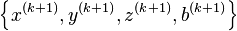
from equations 7 into equations 2, set in equations 7, and reevaluate the residuals in equations 2. This procedure is repeated until the residuals are sufficiently small in magnitude.
P(Y) code
Calculating a position with the P(Y) signal is generally similar in concept, assuming one can decrypt it. The encryption is essentially a safety mechanism: if a signal can be successfully decrypted, it is reasonable to assume it is a real signal being sent by a GPS satellite.[citation needed] In comparison, civil receivers are highly vulnerable to spoofing since correctly formatted C/A signals can be generated using readily available signal generators. RAIM features do not protect against spoofing, since RAIM only checks the signals from a navigational perspective.
Error sources and analysis

| Source | Effect |
|---|---|
| Signal Arrival C/A | ± 3 m |
| Signal Arrival P(Y) | ± 0.3 m |
| Ionospheric effects | ± 5 m |
| Ephemeris errors | ± 2.5 m |
| Satellite clock errors | ± 2 m |
| Multipath distortion | ± 1 m |
| Tropospheric effects | ± 0.5 m |
 C/A C/A | ± 6,7 m |
| P(Y) | ± 6,0 m |
User equivalent range errors (UERE) are shown in the table. There is also a numerical error with an estimated value,  , of about 1 meter. The standard deviations, , for the coarse/acquisition and precise codes are also shown in the table. These standard deviations are computed by taking the square root of the sum of the squares of the individual components (i.e. RSS for root sum squares). To get the standard deviation of receiver position estimate, these range errors must be multiplied by the appropriate dilution of precision terms and then RSS'ed with the numerical error. Electronics errors are one of several accuracy-degrading effects outlined in the table above. When taken together, autonomous civilian GPS horizontal position fixes are typically accurate to about 15 meters (50 ft). These effects also reduce the more precise P(Y) code's accuracy. However, the advancement of technology means that today, civilian GPS fixes under a clear view of the sky are on average accurate to about 5 meters (16 ft) horizontally.(see summary table near end of "Sources of Errors in GPS")

The term user equivalent range error (UERE) refers to the standard deviation of a component of the error in the distance from receiver to a satellite. The standard deviation of the error in receiver position,  , is computed by multiplying PDOP (Position Dilution Of Precision) by , the standard deviation of the user equivalent range errors. is computed by taking the square root of the sum of the squares of the individual component standard deviations.
PDOP is computed as a function of receiver and satellite positions. Consider the unit vectors pointing from the receiver to the satellites. Connecting the tails of these unit vectors forms a tetrahedron. PDOP is sometimes approximated as being inversely proportional to the tetrahedron volume[45]. Also a more detailed description of how to calculate PDOP is given in the section, Geometric dilution of precision computation (DOP).
is given by 
 for the C/A code. The standard deviation of the error in estimated receiver position, , is given by
 for the C/A code. The error diagram to the right shows the inter relationship of indicated receiver position, true receiver position, and the intersection of the four sphere surfaces.
Signal arrival time measurement
The position calculated by a GPS receiver requires the current time, the position of the satellite and the measured delay of the received signal. The position accuracy is primarily dependent on the satellite position and signal delay.
To measure the delay, the receiver compares the bit sequence received from the satellite with an internally generated version. By comparing the rising and trailing edges of the bit transitions, modern electronics can measure signal offset to within about one percent of a bit pulse width,  , or approximately 10 nanoseconds for the C/A code. Since GPS signals propagate at the speed of light, this represents an error of about 3 meters.
This component of position accuracy can be improved by a factor of 10 using the higher-chiprate P(Y) signal. Assuming the same one percent of bit pulse width accuracy, the high-frequency P(Y) signal results in an accuracy of  or about 30 centimeters.
Atmospheric effects
Inconsistencies of atmospheric conditions affect the speed of the GPS signals as they pass through the Earth's atmosphere, especially the ionosphere. Correcting these errors is a significant challenge to improving GPS position accuracy. These effects are smallest when the satellite is directly overhead and become greater for satellites nearer the horizon since the path through the atmosphere is longer (see airmass). Once the receiver's approximate location is known, a mathematical model can be used to estimate and compensate for these errors.
Ionospheric delay of a microwave signal depends on its frequency. This phenomenon is known as dispersion and can be calculated from measurements of delays for two or more frequency bands, allowing delays at other frequencies to be estimated. [53] Some military and expensive survey-grade civilian receivers calculate atmospheric dispersion from the different delays in the L1 and L2 frequencies, and apply a more precise correction. This can be done in civilian receivers without decrypting the P(Y) signal carried on L2, by tracking the carrier wave instead of the modulated code. To facilitate this on lower cost receivers, a new civilian code signal on L2, called L2C, was added to the Block IIR-M satellites, which was first launched in 2005. It allows a direct comparison of the L1 and L2 signals using the coded signal instead of the carrier wave. (see Atmospheric Effects in "Sources of Errors in GPS")
The effects of the ionosphere generally change slowly, and can be averaged over time. Those for any particular geographical area can be easily calculated by comparing the GPS-measured position to a known surveyed location. This correction is also valid for other receivers in the same general location. Several systems send this information over radio or other links to allow L1-only receivers to make ionospheric corrections. The ionospheric data are transmitted via satellite in Satellite Based Augmentation Systems (SBAS) such as WAAS (available in North America and Hawaii), EGNOS (Europe and Asia) or MSAS (Japan), which transmits it on the GPS frequency using a special pseudo-random noise sequence (PRN), so only one receiver and antenna are required.
Humidity also causes a variable delay, resulting in errors similar to ionospheric delay, but occurring in the troposphere. This effect both is more localized and changes more quickly than ionospheric effects, and is not frequency dependent. These traits make precise measurement and compensation of humidity errors more difficult than ionospheric effects.[citation needed]
Changes in receiver altitude also change the amount of delay, due to the signal passing through less of the atmosphere at higher elevations. Since the GPS receiver computes its approximate altitude, this error is relatively simple to correct, either by applying a function regression or correlating margin of atmospheric error to ambient pressure using a barometric altimeter.[citation needed]
Multipath effects
GPS signals can also be affected by multipath issues, where the radio signals reflect off surrounding terrain; buildings, canyon walls, hard ground, etc. These delayed signals can cause inaccuracy. A variety of techniques, most notably narrow correlator spacing, have been developed to mitigate multipath errors. For long delay multipath, the receiver itself can recognize the wayward signal and discard it. To address shorter delay multipath from the signal reflecting off the ground, specialized antennas (e.g. a choke ring antenna) may be used to reduce the signal power as received by the antenna. Short delay reflections are harder to filter out because they interfere with the true signal, causing effects almost indistinguishable from routine fluctuations in atmospheric delay.
Multipath effects are much less severe in moving vehicles. When the GPS antenna is moving, the false solutions using reflected signals quickly fail to converge and only the direct signals result in stable solutions.
Ephemeris and clock errors
While the ephemeris data is transmitted every 30 seconds, the information itself may be up to two hours old. If a fast time to first fix (TTFF) is needed, it is possible to upload a valid ephemeris to a receiver, and in addition to setting the time, a position fix can be obtained in under ten seconds. It is feasible to put such ephemeris data on the web so it can be loaded into mobile GPS devices.[54] See also Assisted GPS.
The satellite's atomic clocks experience noise and clock drift errors. The navigation message contains corrections for these errors and estimates of the accuracy of the atomic clock. However, they are based on observations and may not indicate the clock's current state.
These problems tend to be very small, but may add up to a few meters (10s of feet) of inaccuracy.[55]
For very precise positioning - e.g. in geodesy - these effects can be eliminated by differential GPS: the simultaneous use of two or more receivers at several survey points. In the 1990s when receivers were quite expensive, some methods of quasi-differential GPS were developed, using only one receiver but reoccupation of measuring points. At the TU Vienna the method was named qGPS and adequate software of post processing was developed.
Geometric dilution of precision computation (DOP)
The concept of geometric dilution of precision was introduced in the section, "Error sources and analysis". Computations were provided to show how PDOP was used and how it effected the receiver position error standard deviation.
When visible GPS satellites are close together in the sky (i.e. small angular separation), the DOP values are high; when far apart, the DOP values are low. Thus low DOP values represents a better GPS positional accuracy due to the wider angular separation between the satellites used to calculate a GPS unit's position. DOP can be expressed as a number of separate measurements. HDOP, VDOP, PDOP and TDOP are respectively Horizontal, Vertical, Position (3-D) and Time Dilution of Precision.
Figure 3.1 Dilution of Precision of [17] provide a graphical indication of how geometry affect accuracy.
We now take on the task of how to compute the dilution of precision terms. As a first step in computing DOP, consider the unit vector from the receiver to satellite i with components,
 where the distance from receiver to the satellite,
  , is given by
 and where
  denote the position of the receiver and
  denote the position of satellite i. These x, y, and z components may be components in a North, East, Down coordinate system a South, East, Up coordinate system or other convenient system. Formulate the matrix A as
The first three elements of each row of A are the components of a unit vector from the receiver to the indicated satellite. The elements in the fourth column are c where c denotes the speed of light. Formulate the matrix, Q, as

This computation is in accordance with "Section 1.4.2 of PRINCIPLES OF SATELLITE POSITIONING" where the weighting matrix, P, has been set to the identity matrix.
The elements of the Q matrix are designated as

The Greek letter  is used quite often where we have used d. However the elements of the Q matrix do not represent variances and covariances as they are defined in probability and statistics. Instead they are strictly geometric terms. Therefore d as in dilution of precision is used. PDOP, TDOP and GDOP are given by
 ,
, , and
, and in agreement with "Section 1.4.9 of PRINCIPLES OF SATELLITE POSITIONING".
The horizontal dilution of precision,  , and the vertical dilution of precision,
  , are both dependent on the coordinate system used. To correspond to the local horizon plane and the local vertical, x, y, and z should denote positions in either a North, East, Down coordinate system or a South, East, Up coordinate system.
Derivation of DOP equations
The equations for computing the geometric dilution of precision terms have been described in the previous section. This section describes the derivation of these equations. The method used here is similar to that used in "Global Positioning System (preview) by Parkinson and Spiker"
Consider the position error vector,  , defined as the vector from the intersection of the four sphere surfaces corresponding to the pseudoranges to the true position of the receiver.
  where bold denotes a vector and
  denote unit vectors along the x, y, and z axes respectively. Let
  denote the time error, the true time minus the receiver indicated time. Assume that the mean value of the three components of and are zero.

where  are the errors in pseudoranges 1 through 4 respectively. This equation comes from linearizing the equation relating pseudoranges to receiver position, satellite positions, and receiver clock errors as shown in [2] . Multiplying both sides by
  there results
 .
.
Transposing both sides
 .
.
Post multiplying the matrices on both sides of equation (2) by the corresponding matrices in equation (3), there results
 .
.
Taking the expected value of both sides and taking the non-random matrices outside the expectation operator, E, there results
 .
.
Assuming the pseudorange errors are uncorrelated and have the same variance, the covariance matrix on the right side can be expressed as a scalar times the identity matrix. Thus
since 
Note:  since
since 
Substituting for  there follows

From equation (7), it follows that the variances of indicated receiver position and time are
 and
and .
.
The remaining position and time error variance terms follow in a straightforward manner.
Selective availability
GPS includes a (currently disabled) feature called Selective Availability (SA) that adds intentional, time varying errors of up to 100 meters (328 ft) to the publicly available navigation signals. This was intended to deny an enemy the use of civilian GPS receivers for precision weapon guidance.
SA errors are actually pseudorandom, generated by a cryptographic algorithm from a classified seed key available only to authorized users (the US military, its allies and a few other users, mostly government) with a special military GPS receiver. Mere possession of the receiver is insufficient; it still needs the tightly controlled daily key.
Before it was turned off on May 1, 2000, typical SA errors were 10 meters (32 ft) horizontally and 30 meters (98 ft) vertically. Because SA affects every GPS receiver in a given area almost equally, a fixed station with an accurately known position can measure the SA error values and transmit them to the local GPS receivers so they may correct their position fixes. This is called Differential GPS or DGPS. DGPS also corrects for several other important sources of GPS errors, particularly ionospheric delay, so it continues to be widely used even though SA has been turned off. The ineffectiveness of SA in the face of widely available DGPS was a common argument for turning off SA, and this was finally done by order of President Clinton in 2000.
Another restriction on GPS, antispoofing, remains on. This encrypts the P-code so that it cannot be mimicked by an enemy transmitter sending false information. Few civilian receivers have ever used the P-code, and the accuracy attainable with the public C/A code is so much better than originally expected (especially with DGPS) that the antispoof policy has relatively little effect on most civilian users. Turning off antispoof would primarily benefit surveyors and some scientists who need extremely precise positions for experiments such as tracking the motion of a tectonic plate.
DGPS services are widely available from both commercial and government sources. The latter include WAAS and the US Coast Guard's network of LF marine navigation beacons. The accuracy of the corrections depends on the distance between the user and the DGPS receiver. As the distance increases, the errors at the two sites will not correlate as well, resulting in less precise differential corrections.
During the 1990-91 Gulf War, the shortage of military GPS units caused many troops and their families to buy readily available civilian units. This significantly impeded the US military's own battlefield use of GPS, so the military made the decision to turn off SA for the duration of the war.
In the 1990s, the FAA started pressuring the military to turn off SA permanently. This would save the FAA millions of dollars every year in maintenance of their own radio navigation systems. The amount of error added was "set to zero"[56] at midnight on May 1, 2000 following an announcement by U.S. President Bill Clinton, allowing users access to the error-free L1 signal. Per the directive, the induced error of SA was changed to add no error to the public signals (C/A code). Clinton's executive order required SA to be set to zero by 2006; it happened in 2000 once the US military developed a new system that provides the ability to deny GPS (and other navigation services) to hostile forces in a specific area of crisis without affecting the rest of the world or its own military systems.[56]
Selective Availability is still a system capability of GPS, and error could, in theory, be reintroduced at any time. In practice, in view of the hazards and costs this would induce for US and foreign shipping, it is unlikely to be reintroduced, and various government agencies, including the FAA,[57] have stated that it is not intended to be reintroduced.
One interesting side effect of the Selective Availability hardware is the capability to correct the frequency of the GPS cesium and rubidium atomic clocks to an accuracy of approximately 2 × 10⁻¹³ (one in five trillion). This represented a significant improvement over the raw accuracy of the clocks.[citation needed]
On 19 September 2007, the United States Department of Defense announced that future GPS III satellites will not be capable of implementing SA,[58] eventually making the policy permanent.[59]
Relativity

A number of sources of error exist due to relativistic effects.[60] For example, the relativistic time slowing due to the speed of the satellite of about 1 part in 1010, the gravitational time dilation that makes a satellite run about 5 parts in 1010 faster than an Earth based clock, and the Sagnac effect due to rotation relative to receivers on Earth. These topics are examined below, one at a time.
Special and general relativity
According to the theory of relativity, due to their constant movement and height relative to the Earth-centered, non-rotating approximately inertial reference frame, the clocks on the satellites are affected by their speed (special relativity) Special relativity predicts that atomic clocks moving at GPS orbital speeds will tick more slowly than stationary ground clocks by about 7.2 μs per day.
For the GPS satellites, general relativity predicts that the atomic clocks at GPS orbital altitudes will tick more rapidly, by about 45.9 microseconds (μs) per day, because they have a higher gravitational potential than atomic clocks on Earth's surface.
When combined, the discrepancy is about 38 microseconds per day; a difference of 4.465 parts in 1010.[61] To account for this discrepancy, the frequency standard on board each satellite is given a rate offset prior to launch, making it run slightly slower than the desired frequency on Earth; specifically, at 10.22999999543 MHz instead of 10.23 MHz.[62] Since the atomic clocks on board the GPS satellites are precisely tuned, it makes the system a practical engineering application of the scientific theory of relativity in a real-world environment. Placing atomic clocks on artificial satellites to test Einstein's general theory was proposed by Friedwardt Winterberg in 1955.[63][verification needed]
Sagnac distortion
GPS observation processing must also compensate for the Sagnac effect. The GPS time scale is defined in an inertial system but observations are processed in an Earth-centered, Earth-fixed (co-rotating) system, a system in which simultaneity is not uniquely defined. A Lorentz transformation is thus applied to convert from the inertial system to the ECEF system. The resulting signal run time correction has opposite algebraic signs for satellites in the Eastern and Western celestial hemispheres. Ignoring this effect will produce an east-west error on the order of hundreds of nanoseconds, or tens of meters in position.[64]
Natural sources of interference
Since GPS signals at terrestrial receivers tend to be relatively weak, natural radio signals or scattering of the GPS signals can desensitize the receiver, making acquiring and tracking the satellite signals difficult or impossible.
Space weather degrades GPS operation in two ways, direct interference by solar radio burst noise in the same frequency band [65] or by scattering of the GPS radio signal in ionospheric irregularities referred to as scintillation [66]. Both forms of degradation follow the 11 year solar cycle and are a maximum at sunspot maximum although they can occur at anytime. Solar radio bursts are associated with solar flares and their impact can affect reception over the half of the Earth facing the sun. Scintillation occurs most frequently at tropical latitudes where it is a night time phenomenon. It occurs less frequently at high latitudes or mid-latitudes where magnetic storms can lead to scintillation [67]. In addition to producing scintillation, magnetic storms can produce strong ionospheric gradients that degrade the accuracy of SBAS systems [68].
Artificial sources of interference
In automotive GPS receivers, metallic features in windshields,[69] such as defrosters, or car window tinting films[70] can act as a Faraday cage, degrading reception just inside the car.
Man-made EMI (electromagnetic interference) can also disrupt, or jam, GPS signals. In one well documented case, the entire harbor of Moss Landing, California was unable to receive GPS signals due to unintentional jamming caused by malfunctioning TV antenna preamplifiers.[71][72] Intentional jamming is also possible. Generally, stronger signals can interfere with GPS receivers when they are within radio range, or line of sight. In 2002, a detailed description of how to build a short range GPS L1 C/A jammer was published in the online magazine Phrack.[73]
The U.S. government believes that such jammers were used occasionally during the 2001 war in Afghanistan and the U.S. military claimed to destroy six GPS jammers during the Iraq War, including one that was destroyed ironically with a GPS-guided bomb.[74] Such a jammer is relatively easy to detect and locate, making it an attractive target for anti-radiation missiles. The UK Ministry of Defence tested a jamming system in the UK's West Country on 7 and 8 June 2007.[75]
Some countries allow the use of GPS repeaters to allow for the reception of GPS signals indoors and in obscured locations, however, under EU and UK laws, the use of these is prohibited as the signals can cause interference to other GPS receivers that may receive data from both GPS satellites and the repeater.
Due to the potential for both natural and man-made noise, numerous techniques continue to be developed to deal with the interference. The first is to not rely on GPS as a sole source. According to John Ruley, "IFR pilots should have a fallback plan in case of a GPS malfunction".[76] Receiver Autonomous Integrity Monitoring (RAIM) is a feature now included in some receivers, which is designed to provide a warning to the user if jamming or another problem is detected. The U.S. military has also deployed their Selective Availability / Anti-Spoofing Module (SAASM) in the Defense Advanced GPS Receiver (DAGR). In demonstration videos, the DAGR is able to detect jamming and maintain its lock on the encrypted GPS signals during interference which causes civilian receivers to lose lock.[77]
Accuracy enhancement
Augmentation
Augmentation methods of improving accuracy rely on external information being integrated into the calculation process. There are many such systems in place and they are generally named or described based on how the GPS sensor receives the information. Some systems transmit additional information about sources of error (such as clock drift, ephemeris, or ionospheric delay), others provide direct measurements of how much the signal was off in the past, while a third group provide additional navigational or vehicle information to be integrated in the calculation process.
Examples of augmentation systems include the Wide Area Augmentation System, Differential GPS, Inertial Navigation Systems and Assisted GPS.
Precise monitoring
The accuracy of a calculation can also be improved through precise monitoring and measuring of the existing GPS signals in additional or alternate ways.
After SA, which has been turned off, the largest error in GPS is usually the unpredictable delay through the ionosphere. The spacecraft broadcast ionospheric model parameters, but errors remain. This is one reason the GPS spacecraft transmit on at least two frequencies, L1 and L2. Ionospheric delay is a well-defined function of frequency and the total electron content (TEC) along the path, so measuring the arrival time difference between the frequencies determines TEC and thus the precise ionospheric delay at each frequency.
Receivers with decryption keys can decode the P(Y)-code transmitted on both L1 and L2. However, these keys are reserved for the military and "authorized" agencies and are not available to the public. Without keys, it is still possible to use a codeless technique to compare the P(Y) codes on L1 and L2 to gain much of the same error information. However, this technique is slow, so it is currently limited to specialized surveying equipment. In the future, additional civilian codes are expected to be transmitted on the L2 and L5 frequencies (see GPS modernization, below). Then all users will be able to perform dual-frequency measurements and directly compute ionospheric delay errors.
A second form of precise monitoring is called Carrier-Phase Enhancement (CPGPS). The error, which this corrects, arises because the pulse transition of the PRN is not instantaneous, and thus the correlation (satellite-receiver sequence matching) operation is imperfect. The CPGPS approach utilizes the L1 carrier wave, which has a period one one-thousandth of the C/A bit period, to act as an additional clock signal and resolve the uncertainty. The phase difference error in the normal GPS amounts to between 2 and 3 meters (6 to 10 ft) of ambiguity. CPGPS working to within 1% of perfect transition reduces this error to 3 centimeters (1 inch) of ambiguity. By eliminating this source of error, CPGPS coupled with DGPS normally realizes between 20 and 30 centimeters (8 to 12 inches) of absolute accuracy.
Relative Kinematic Positioning (RKP) is another approach for a precise GPS-based positioning system. In this approach, determination of range signal can be resolved to a precision of less than 10 centimeters (4 in). This is done by resolving the number of cycles in which the signal is transmitted and received by the receiver. This can be accomplished by using a combination of differential GPS (DGPS) correction data, transmitting GPS signal phase information and ambiguity resolution techniques via statistical tests—possibly with processing in real-time (real-time kinematic positioning, RTK).
Timekeeping
While most clocks are synchronized to Coordinated Universal Time (UTC), the atomic clocks on the satellites are set to GPS time. The difference is that GPS time is not corrected to match the rotation of the Earth, so it does not contain leap seconds or other corrections which are periodically added to UTC. GPS time was set to match Coordinated Universal Time (UTC) in 1980, but has since diverged. The lack of corrections means that GPS time remains at a constant offset with International Atomic Time (TAI)(TAI - GPS = 19 seconds). Periodic corrections are performed on the on-board clocks to correct relativistic effects and keep them synchronized with ground clocks.
The GPS navigation message includes the difference between GPS time and UTC, which as of 2009 is 15 seconds due to the leap second added to UTC December 31 2008. Receivers subtract this offset from GPS time to calculate UTC and specific timezone values. New GPS units may not show the correct UTC time until after receiving the UTC offset message. The GPS-UTC offset field can accommodate 255 leap seconds (eight bits) which, given the current rate of change of the Earth's rotation (with one leap second introduced approximately every 18 months), should be sufficient to last until approximately year 2300.
As opposed to the year, month, and day format of the Gregorian calendar, the GPS date is expressed as a week number and a seconds-into-week number. The week number is transmitted as a ten-bit field in the C/A and P(Y) navigation messages, and so it becomes zero again every 1,024 weeks (19.6 years). GPS week zero started at 00:00:00 UTC (00:00:19 TAI) on January 6 1980, and the week number became zero again for the first time at 23:59:47 UTC on August 21 1999 (00:00:19 TAI on August 22 1999). To determine the current Gregorian date, a GPS receiver must be provided with the approximate date (to within 3,584 days) to correctly translate the GPS date signal. To address this concern the modernized GPS navigation message uses a 13-bit field, which only repeats every 8,192 weeks (157 years), thus lasting until year 2137 (157 years after GPS week zero).
Applications
The Global Positioning System, while originally a military project, is considered a dual-use technology, meaning it has significant applications for both the military and the civilian industry.
Military
The military applications of GPS span many purposes:
- Navigation: GPS allows soldiers to find objectives in the dark or in unfamiliar territory, and to coordinate the movement of troops and supplies. The GPS-receivers that commanders and soldiers use are respectively called the Commanders Digital Assistant and the Soldier Digital Assistant.[78][79][80][81]
- Target tracking: Various military weapons systems use GPS to track potential ground and air targets before they are flagged as hostile.[citation needed] These weapon systems pass GPS co-ordinates of targets to precision-guided munitions to allow them to engage the targets accurately. Military aircraft, particularly those used in air-to-ground roles use GPS to find targets (for example, gun camera video from AH-1 Cobras in Iraq show GPS co-ordinates that can be looked up in Google Earth).
- Missile and projectile guidance: GPS allows accurate targeting of various military weapons including ICBMs, cruise missiles and precision-guided munitions. Artillery projectiles with embedded GPS receivers able to withstand accelerations of 12,000 g's or about
 have been developed for use in 155 mm howitzers.[82]
 - Search and Rescue: Downed pilots can be located faster if they have a GPS receiver.
- Reconnaissance and Map Creation: The military use GPS extensively to aid mapping and reconnaissance.
- The GPS satellites also carry a set of nuclear detonation detectors consisting of an optical sensor (Y-sensor), an X-ray sensor, a dosimeter, and an Electro-Magnetic Pulse (EMP) sensor (W-sensor) which form a major portion of the United States Nuclear Detonation Detection System.[83][84]
Civilian

Many civilian applications benefit from GPS signals, using one or more of three basic components of the GPS: absolute location, relative movement, and time transfer.
The ability to determine the receiver's absolute location allows GPS receivers to perform as a surveying tool or as an aid to navigation. The capacity to determine relative movement enables a receiver to calculate local velocity and orientation, useful in vessels or observations of the Earth. Being able to synchronize clocks to exacting standards enables time transfer, which is critical in large communication and observation systems. An example is CDMA digital cellular. Each base station has a GPS timing receiver to synchronize its spreading codes with other base stations to facilitate inter-cell hand off and support hybrid GPS/CDMA positioning of mobiles for emergency calls and other applications. Finally, GPS enables researchers to explore the Earth environment including the atmosphere, ionosphere and gravity field. GPS survey equipment has revolutionized tectonics by directly measuring the motion of faults in earthquakes.
The Government controls the export of some civilian receivers. All GPS receivers capable of functioning above 18 km (60,000 ft) altitude and 515 m/s (1,000 knots) [85] are classified as munitions (weapons) for which US State Department export licenses are required. These parameters are clearly chosen to prevent use of a receiver in a ballistic missile. It would not prevent use in a cruise missile since their altitudes and speeds are similar to those of ordinary aircraft.
This rule applies even to otherwise purely civilian units that only receive the L1 frequency and the C/A code and cannot correct for SA, etc.
Disabling operation above these limits exempts the receiver from classification as a munition. Different vendors have interpreted these limitations differently. The rule specifies operation above 18 km and 515 m/s, but some receivers stop operating at 18 km even when stationary. This has caused problems with some amateur radio balloon launches as they regularly reach 100,000 feet (30 km).
GPS tours are also an example of civilian use. The GPS is used to determine which content to display. For instance, when approaching a monument it would tell you about the monument.
GPS functionality has now started to move into mobile phones en masse. The first handsets with integrated GPS were launched already in the late 1990’s, and were available for broader consumer availability on networks such as those run by Nextel, Sprint and Verizon in 2002 in response to US FCC mandates for handset positioning in emergency calls. Capabilities for access by third party software developers to these features were slower in coming, with Nextel opening up those APIs upon launch to any developer, Sprint following in 2006, and Verizon soon thereafter.
Awards
Two GPS developers received the National Academy of Engineering Charles Stark Draper Prize for 2003:
- Ivan Getting, emeritus president of The Aerospace Corporation and engineer at the Massachusetts Institute of Technology, established the basis for GPS, improving on the World War II land-based radio system called LORAN (Long-range Radio Aid to Navigation).
- Bradford Parkinson, professor of aeronautics and astronautics at Stanford University, conceived the present satellite-based system in the early 1960s and developed it in conjunction with the U.S. Air Force. Parkinson served twenty-one years in the Air Force, from 1957 to 1978, and retired with the rank of colonel.
One GPS developer, Roger L. Easton, received the National Medal of Technology on February 13, 2006 at the White House.[86]
On February 10, 1993, the National Aeronautic Association selected the Global Positioning System Team as winners of the 1992 Robert J. Collier Trophy, the most prestigious aviation award in the United States. This team consists of researchers from the Naval Research Laboratory, the U.S. Air Force, the Aerospace Corporation, Rockwell International Corporation, and IBM Federal Systems Company. The citation accompanying the presentation of the trophy honors the GPS Team "for the most significant development for safe and efficient navigation and surveillance of air and spacecraft since the introduction of radio navigation 50 years ago."